Hot Notes: 2013

From Wikipedia, the free encyclopedia

Jump to: navigation, search

For the soul music group, see The Vibrations. For the machining context, see Machining vibrations.

For other uses, see Vibrations (disambiguation).

Classical mechanics
History of classical mechanics Timeline of classical mechanics
Branches[show]
Formulations[show]
Fundamental concepts[show]
Core topics[show]
Scientists[show]
v t e

Vibration is a mechanical phenomenon whereby oscillations occur about an equilibrium point. The oscillations may be periodic such as the motion of a pendulum or random such as the movement of a tire on a gravel road.
Vibration is occasionally "desirable". For example the motion of a tuning fork, the reed in a woodwind instrument or harmonica, or mobile phones or the cone of a loudspeaker is desirable vibration, necessary for the correct functioning of the various devices.
More often, vibration is undesirable, wasting energy and creating unwanted sound – noise. For example, the vibrational motions of engines, electric motors, or any mechanical device in operation are typically unwanted. Such vibrations can be caused by imbalances in the rotating parts, uneven friction, the meshing of gear teeth, etc. Careful designs usually minimize unwanted vibrations.
The study of sound and vibration are closely related. Sound, or "pressure waves", are generated by vibrating structures (e.g. vocal cords); these pressure waves can also induce the vibration of structures (e.g. ear drum). Hence, when trying to reduce noise it is often a problem in trying to reduce vibration.

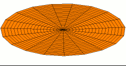
One of the possible modes of vibration of a circular drum (see other modes).

One of the possible modes of vibration of a cantilevered I-beam.

1 Types of vibration
2 Vibration testing
3 Vibration analysis
- 3.1 Free vibration without damping
  - 3.1.1 What causes the system to vibrate: from conservation of energy point of view
- 3.2 Free vibration with damping
  - 3.2.1 Damped and undamped natural frequencies
- 3.3 Forced vibration with damping
  - 3.3.1 What causes resonance?
  - 3.3.2 Applying "complex" forces to the mass–spring–damper model
  - 3.3.3 Frequency response model
4 Multiple degrees of freedom systems and mode shapes
- 4.1 Eigenvalue problem
- 4.2 Illustration of a multiple DOF problem
- 4.3 Multiple DOF problem converted to a single DOF problem
5 See also
6 References
7 Further reading
8 External links

Types of vibration

Free vibration occurs when a mechanical system is set off with an initial input and then allowed to vibrate freely. Examples of this type of vibration are pulling a child back on a swing and then letting go or hitting a tuning fork and letting it ring. The mechanical system will then vibrate at one or more of its "natural frequency" and damp down to zero.
Forced vibration is when an alternating force or motion is applied to a mechanical system. Examples of this type of vibration include a shaking washing machine due to an imbalance, transportation vibration (caused by truck engine, springs, road, etc.), or the vibration of a building during an earthquake. In forced vibration the frequency of the vibration is the frequency of the force or motion applied, with order of magnitude being dependent on the actual mechanical system.

Vibration testing

Vibration testing is accomplished by introducing a forcing function into a structure, usually with some type of shaker.^[1] Alternately, a DUT (device under test) is attached to the "table" of a shaker. For relatively low frequency forcing, servohydraulic (electrohydraulic) shakers are used. For higher frequencies, electrodynamic shakers are used. Generally, one or more "input" or "control" points located on the DUT-side of a fixture is kept at a specified acceleration.^[2] Other "response" points experience maximum vibration level (resonance) or minimum vibration level (anti-resonance).
Two typical types of vibration tests performed are random- and sine test. Sine (one-frequency-at-a-time) tests are performed to survey the structural response of the device under test (DUT). A random (all frequencies at once) test is generally considered to more closely replicate a real world environment, such as road inputs to a moving automobile.
Most vibration testing is conducted in a single DUT axis at a time, even though most real-world vibration occurs in various axes simultaneously. MIL-STD-810G, released in late 2008, Test Method 527, calls for multiple exciter testing.

Vibration analysis

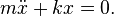
The fundamentals of vibration analysis can be understood by studying the simple mass–spring–damper model. Indeed, even a complex structure such as an automobile body can be modeled as a "summation" of simple mass–spring–damper models. The mass–spring–damper model is an example of a simple harmonic oscillator. The mathematics used to describe its behavior is identical to other simple harmonic oscillators such as the RLC circuit.
Note: In this article the step by step mathematical derivations will not be included, but will focus on the major equations and concepts in vibration analysis. Please refer to the references at the end of the article for detailed derivations.

Free vibration without damping

To start the investigation of the mass–spring–damper we will assume the damping is negligible and that there is no external force applied to the mass (i.e. free vibration). The force applied to the mass by the spring is proportional to the amount the spring is stretched "x" (we will assume the spring is already compressed due to the weight of the mass). The proportionality constant, k, is the stiffness of the spring and has units of force/distance (e.g. lbf/in or N/m). The negative sign indicates that the force is always opposing the motion of the mass attached to it:

$F_s=- k x. \!$

The force generated by the mass is proportional to the acceleration of the mass as given by Newton’s second law of motion :

$\Sigma\ F = ma = m \ddot{x} = m \frac{d^2x}{dt^2}.$

The sum of the forces on the mass then generates this ordinary differential equation: $\ m \ddot{x} + k x = 0.$

Simple harmonic motion of the mass–spring system

If we assume that we start the system to vibrate by stretching the spring by the distance of A and letting go, the solution to the above equation that describes the motion of mass is:

$x(t) = A \cos (2 \pi f_n t). \!$

This solution says that it will oscillate with simple harmonic motion that has an amplitude of A and a frequency of f_n. The number f_n is one of the most important quantities in vibration analysis and is called the undamped natural frequency. For the simple mass–spring system, f_n is defined as:

$f_n = {1\over {2 \pi}} \sqrt{k \over m}. \!$

Note: Angular frequency ω (ω=2 π f) with the units of radians per second is often used in equations because it simplifies the equations, but is normally converted to “standard” frequency (units of Hz or equivalently cycles per second) when stating the frequency of a system. If you know the mass and stiffness of the system you can determine the frequency at which the system will vibrate once it is set in motion by an initial disturbance using the above stated formula. Every vibrating system has one or more natural frequencies that it will vibrate at once it is disturbed. This simple relation can be used to understand in general what will happen to a more complex system once we add mass or stiffness. For example, the above formula explains why when a car or truck is fully loaded the suspension will feel ″softer″ than unloaded because the mass has increased and therefore reduced the natural frequency of the system.

What causes the system to vibrate: from conservation of energy point of view

Vibrational motion could be understood in terms of conservation of energy. In the above example we have extended the spring by a value of x and therefore have stored some potential energy (\tfrac {1}{2} k x^2) in the spring. Once we let go of the spring, the spring tries to return to its un-stretched state (which is the minimum potential energy state) and in the process accelerates the mass. At the point where the spring has reached its un-stretched state all the potential energy that we supplied by stretching it has been transformed into kinetic energy (\tfrac {1}{2} m v^2). The mass then begins to decelerate because it is now compressing the spring and in the process transferring the kinetic energy back to its potential. Thus oscillation of the spring amounts to the transferring back and forth of the kinetic energy into potential energy. In our simple model the mass will continue to oscillate forever at the same magnitude, but in a real system there is always something called damping that dissipates the energy, eventually bringing it to rest.

Free vibration with damping

Mass Spring Damper Model

We now add a "viscous" damper to the model that outputs a force that is proportional to the velocity of the mass. The damping is called viscous because it models the effects of an object within a fluid. The proportionality constant c is called the damping coefficient and has units of Force over velocity (lbf s/ in or N s/m).

$F_d = - c v = - c \dot{x} = - c \frac{dx}{dt}. \!$

By summing the forces on the mass we get the following ordinary differential equation:

$m \ddot{x} + { c } \dot{x} + {k } x = 0.$

The solution to this equation depends on the amount of damping. If the damping is small enough the system will still vibrate, but eventually, over time, will stop vibrating. This case is called underdamping – this case is of most interest in vibration analysis. If we increase the damping just to the point where the system no longer oscillates we reach the point of critical damping (if the damping is increased past critical damping the system is called overdamped). The value that the damping coefficient needs to reach for critical damping in the mass spring damper model is:

$c_c= 2 \sqrt{k m}.$

To characterize the amount of damping in a system a ratio called the damping ratio (also known as damping factor and % critical damping) is used. This damping ratio is just a ratio of the actual damping over the amount of damping required to reach critical damping. The formula for the damping ratio ( $\zeta$ ) of the mass spring damper model is:

$\zeta = { c \over 2 \sqrt{k m} }.$

For example, metal structures (e.g. airplane fuselage, engine crankshaft) will have damping factors less than 0.05 while automotive suspensions in the range of 0.2–0.3.
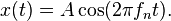
The solution to the underdamped system for the mass spring damper model is the following:

$x(t)=X e^{-\zeta \omega_n t} \cos({\sqrt{1-\zeta^2} \omega_n t - \phi}) , \qquad \omega_n= 2\pi f_n.$

The value of X, the initial magnitude, and $\phi,$ the phase shift, are determined by the amount the spring is stretched. The formulas for these values can be found in the references.

Damped and undamped natural frequencies

The major points to note from the solution are the exponential term and the cosine function. The exponential term defines how quickly the system “damps” down – the larger the damping ratio, the quicker it damps to zero. The cosine function is the oscillating portion of the solution, but the frequency of the oscillations is different from the undamped case.
The frequency in this case is called the "damped natural frequency", $f_d,$ and is related to the undamped natural frequency by the following formula:

$f_d= f_n\sqrt{1-\zeta^2}.\,$

The damped natural frequency is less than the undamped natural frequency, but for many practical cases the damping ratio is relatively small and hence the difference is negligible. Therefore the damped and undamped description are often dropped when stating the natural frequency (e.g. with 0.1 damping ratio, the damped natural frequency is only 1% less than the undamped).
The plots to the side present how 0.1 and 0.3 damping ratios effect how the system will “ring” down over time. What is often done in practice is to experimentally measure the free vibration after an impact (for example by a hammer) and then determine the natural frequency of the system by measuring the rate of oscillation as well as the damping ratio by measuring the rate of decay. The natural frequency and damping ratio are not only important in free vibration, but also characterize how a system will behave under forced vibration.

Forced vibration with damping

In this section we will see the behavior of the spring mass damper model when we add a harmonic force in the form below. A force of this type could, for example, be generated by a rotating imbalance.

$F= F_0 \cos {(2 \pi f t)}. \!$

If we again sum the forces on the mass we get the following ordinary differential equation:

$m \ddot{x} + { c } \dot{x} + {k } x = F_0 \cos {(2 \pi f t)}.$

The steady state solution of this problem can be written as:

$x(t)= X \cos {(2 \pi f t -\phi)}. \!$

The result states that the mass will oscillate at the same frequency, f, of the applied force, but with a phase shift $\phi.$
The amplitude of the vibration “X” is defined by the following formula.

$X= {F_0 \over k} {1 \over \sqrt{(1-r^2)^2 + (2 \zeta r)^2}}.$

Where “r” is defined as the ratio of the harmonic force frequency over the undamped natural frequency of the mass–spring–damper model.

$r=\frac{f}{f_n}.$

The phase shift, $\phi,$ is defined by the following formula.

$\phi= \arctan {\left (\frac{2 \zeta r}{1-r^2} \right)}.$

The plot of these functions, called "the frequency response of the system", presents one of the most important features in forced vibration. In a lightly damped system when the forcing frequency nears the natural frequency ( $r \approx 1$ ) the amplitude of the vibration can get extremely high. This phenomenon is called resonance (subsequently the natural frequency of a system is often referred to as the resonant frequency). In rotor bearing systems any rotational speed that excites a resonant frequency is referred to as a critical speed.
If resonance occurs in a mechanical system it can be very harmful – leading to eventual failure of the system. Consequently, one of the major reasons for vibration analysis is to predict when this type of resonance may occur and then to determine what steps to take to prevent it from occurring. As the amplitude plot shows, adding damping can significantly reduce the magnitude of the vibration. Also, the magnitude can be reduced if the natural frequency can be shifted away from the forcing frequency by changing the stiffness or mass of the system. If the system cannot be changed, perhaps the forcing frequency can be shifted (for example, changing the speed of the machine generating the force).
The following are some other points in regards to the forced vibration shown in the frequency response plots.

At a given frequency ratio, the amplitude of the vibration, X, is directly proportional to the amplitude of the force $F_0$ (e.g. if you double the force, the vibration doubles)
With little or no damping, the vibration is in phase with the forcing frequency when the frequency ratio r < 1 and 180 degrees out of phase when the frequency ratio r > 1
When r ≪ 1 the amplitude is just the deflection of the spring under the static force $F_0.$ This deflection is called the static deflection $\delta_{st}.$ Hence, when r ≪ 1 the effects of the damper and the mass are minimal.
When r ≫ 1 the amplitude of the vibration is actually less than the static deflection $\delta_{st}.$ In this region the force generated by the mass (F = ma) is dominating because the acceleration seen by the mass increases with the frequency. Since the deflection seen in the spring, X, is reduced in this region, the force transmitted by the spring (F = kx) to the base is reduced. Therefore the mass–spring–damper system is isolating the harmonic force from the mounting base – referred to as vibration isolation. Interestingly, more damping actually reduces the effects of vibration isolation when r ≫ 1 because the damping force (F = cv) is also transmitted to the base.
whatever the damping is , the vibration is 90 degrees out of phase with the forcing frequency when the frequency ratio r =1 ,which is very helpful when it comes to determining the natural frequency of the system.
whatever the damping is ,when r ≫1, the vibration is 180 degrees out of phase with the forcing frequency
whatever the damping is ,when r ≪ 1, the vibration is in phase with the forcing frequency

What causes resonance?

Resonance is simple to understand if you view the spring and mass as energy storage elements – with the mass storing kinetic energy and the spring storing potential energy. As discussed earlier, when the mass and spring have no external force acting on them they transfer energy back and forth at a rate equal to the natural frequency. In other words, if energy is to be efficiently pumped into both the mass and spring the energy source needs to feed the energy in at a rate equal to the natural frequency. Applying a force to the mass and spring is similar to pushing a child on swing, you need to push at the correct moment if you want the swing to get higher and higher. As in the case of the swing, the force applied does not necessarily have to be high to get large motions; the pushes just need to keep adding energy into the system.
The damper, instead of storing energy, dissipates energy. Since the damping force is proportional to the velocity, the more the motion, the more the damper dissipates the energy. Therefore a point will come when the energy dissipated by the damper will equal the energy being fed in by the force. At this point, the system has reached its maximum amplitude and will continue to vibrate at this level as long as the force applied stays the same. If no damping exists, there is nothing to dissipate the energy and therefore theoretically the motion will continue to grow on into infinity.

Applying "complex" forces to the mass–spring–damper model

In a previous section only a simple harmonic force was applied to the model, but this can be extended considerably using two powerful mathematical tools. The first is the Fourier transform that takes a signal as a function of time (time domain) and breaks it down into its harmonic components as a function of frequency (frequency domain). For example, let us apply a force to the mass–spring–damper model that repeats the following cycle – a force equal to 1 newton for 0.5 second and then no force for 0.5 second. This type of force has the shape of a 1 Hz square wave.

How a 1 Hz square wave can be represented as a summation of sine waves(harmonics) and the corresponding frequency spectrum. Click and go to full resolution for an animation

The Fourier transform of the square wave generates a frequency spectrum that presents the magnitude of the harmonics that make up the square wave (the phase is also generated, but is typically of less concern and therefore is often not plotted). The Fourier transform can also be used to analyze non-periodic functions such as transients (e.g. impulses) and random functions. With the advent of the modern computer the Fourier transform is almost always computed using the Fast Fourier Transform (FFT) computer algorithm in combination with a window function.
In the case of our square wave force, the first component is actually a constant force of 0.5 newton and is represented by a value at "0" Hz in the frequency spectrum. The next component is a 1 Hz sine wave with an amplitude of 0.64. This is shown by the line at 1 Hz. The remaining components are at odd frequencies and it takes an infinite amount of sine waves to generate the perfect square wave. Hence, the Fourier transform allows you to interpret the force as a sum of sinusoidal forces being applied instead of a more "complex" force (e.g. a square wave).
In the previous section, the vibration solution was given for a single harmonic force, but the Fourier transform will in general give multiple harmonic forces. The second mathematical tool, "the principle of superposition", allows you to sum the solutions from multiple forces if the system is linear. In the case of the spring–mass–damper model, the system is linear if the spring force is proportional to the displacement and the damping is proportional to the velocity over the range of motion of interest. Hence, the solution to the problem with a square wave is summing the predicted vibration from each one of the harmonic forces found in the frequency spectrum of the square wave.

Frequency response model

We can view the solution of a vibration problem as an input/output relation – where the force is the input and the output is the vibration. If we represent the force and vibration in the frequency domain (magnitude and phase) we can write the following relation:

$X(i\omega)=H(i\omega)\cdot F(i\omega) \ \ or \ \ H(i\omega)= {X(i\omega) \over F(i\omega)}.$

$H(i\omega)$ is called the frequency response function (also referred to as the transfer function, but not technically as accurate) and has both a magnitude and phase component (if represented as a complex number, a real and imaginary component). The magnitude of the frequency response function (FRF) was presented earlier for the mass–spring–damper system.

$|H(i\omega)|=\left |{X(i\omega) \over F(i\omega)} \right|= {1 \over k} {1 \over \sqrt{(1-r^2)^2 + (2 \zeta r)^2}},$ where $r=\frac{f}{f_n}=\frac{\omega}{\omega_n}.$

The phase of the FRF was also presented earlier as:

$\angle H(i\omega)= -\arctan {\left (\frac{2 \zeta r}{1-r^2} \right)}.$

For example, let us calculate the FRF for a mass–spring–damper system with a mass of 1 kg, spring stiffness of 1.93 N/mm and a damping ratio of 0.1. The values of the spring and mass give a natural frequency of 7 Hz for this specific system. If we apply the 1 Hz square wave from earlier we can calculate the predicted vibration of the mass. The figure illustrates the resulting vibration. It happens in this example that the fourth harmonic of the square wave falls at 7 Hz. The frequency response of the mass–spring–damper therefore outputs a high 7 Hz vibration even though the input force had a relatively low 7 Hz harmonic. This example highlights that the resulting vibration is dependent on both the forcing function and the system that the force is applied to.

Frequency response model

The figure also shows the time domain representation of the resulting vibration. This is done by performing an inverse Fourier Transform that converts frequency domain data to time domain. In practice, this is rarely done because the frequency spectrum provides all the necessary information.
The frequency response function (FRF) does not necessarily have to be calculated from the knowledge of the mass, damping, and stiffness of the system, but can be measured experimentally. For example, if you apply a known force and sweep the frequency and then measure the resulting vibration you can calculate the frequency response function and then characterize the system. This technique is used in the field of experimental modal analysis to determine the vibration characteristics of a structure.

Hot Notes

Thursday, 10 January 2013

Vibration

Contents

Types of vibration

Vibration testing

Vibration analysis

Free vibration without damping

What causes the system to vibrate: from conservation of energy point of view

Free vibration with damping

Damped and undamped natural frequencies

Forced vibration with damping

What causes resonance?

Applying "complex" forces to the mass–spring–damper model

Frequency response model

Source : Wikipedia http://en.wikipedia.org/wiki/Vibration

CURSUL BNR: Leul se apreciază semnificativ

Codul rutier 2013 modificat intră în vigoare din 19 ianuarie. Vezi toate schimbările

Wednesday, 9 January 2013

Kingston: Behold the 1-terabyte flash drive





Închide